Reinforcement Learning

Overview

This template is a starting point for building and operating Reinforcement Learning (RL) training and serving on AWS. Using demand and profit optimization as examples, it implements a Deep RL workflow to illustrate the end-to-end ML-Ops framework—covering orchestration, data pipelines, training, evaluation and deployment. The document discusses RL at a high level, but its primary focus is the AWS ML-Ops architecture rather than the algorithms.

Machine Learning is generally classified into three categories: Supervised Learning, Unsupervised Learning, and Reinforcement Learning (RL). RL is a specialized branch of machine learning that focuses on sequential decision-making to maximize cumulative rewards within a given environment. Unlike supervised learning, which relies on labeled datasets with predefined outcomes, RL enables an agent to learn through direct interaction—taking actions in a dynamic environment and refining its strategy based on feedback in the form of rewards or penalties.

In reinforcement learning, an agent learns by interacting with its environment, which provides the current state. Based on this state, the agent selects an action. The environment then returns a reward signal and transitions to a new state. Positive rewards encourage the agent to repeat similar actions in comparable future states, while negative rewards discourage them. By iterating through this cycle—state → action → reward → new state—the agent gradually learns a policy that maximizes cumulative rewards to achieve the specified goal.

Key Concept of Reinforcement Learning

Agent: The learner or decision-maker.
Environment: Everything the agent interacts with.
State: A specific situation in which the agent finds itself.
Action: All possible moves the agent can make.
Reward: Feedback from the environment based on the action taken.

How Reinforcement Learning works

RL operates on the principle of learning optimal behavior through trial and error. The agent takes actions within the environment, receives rewards or penalties, and adjusts its behavior to maximize the cumulative reward. This learning process is characterized by the following elements:

Policy: A strategy used by the agent to determine the next action based on the current state.
Reward Function: A function that provides a scalar feedback signal based on the state and action.
Value Function: A function that estimates the expected cumulative reward from a given state.
Environment: A representation of the environment that helps in planning by predicting future states and rewards.

Deep Reinforcement Learning

Deep reinforcement learning (deep RL) is a subfield of machine learning that combines reinforcement learning (RL) and deep learning. RL considers the problem of a computational agent learning to make decisions by trial and error. Deep RL incorporates deep learning into the solution, allowing agents to make decisions from unstructured input data without manual engineering of the state space. Deep RL algorithms are able to take in very large inputs (e.g. every pixel rendered to the screen in a video game) and decide what actions to perform to optimize an objective (e.g. maximizing the game score). Deep reinforcement learning has been used for a diverse set of applications including but not limited to robotics, video games, natural language processing.

Q-Learning and Deep Q-Learning

Q-learning is a reinforcement learning algorithm that finds an optimal action-selection policy for any finite Markov decision process (MDP). It helps an agent learn to maximize the total reward over time through repeated interactions with the environment, even when the model of that environment is not known.

Vanilla Q-Learning: A table maps each state-action pair to its corresponding Q-value
Deep Q-Learning: A Neural Network maps input states to (action, Q-value) pairs
The diagram below illustrates the conceptual flow of Deep Q-Learning. Through repeated iterations of this process, the algorithm progressively refines its decision-making and converges on an optimal policy, which is represented by a trained neural network.

1.Initialize your Main and Target neural networks
2.Choose an action using the Epsilon-Greedy Exploration Strategy
3.Update your network weights using the Bellman Equation

Bellman Equation

The Bellman Equation: simplify our value estimation – Hugging Face Deep RL Course

In this template, a Deep Q-Learning model is trained to address a demand and profit optimization problem within a simulated, highly simplified environment.

Reinforcement Learning Environment

OpenAI Gym
Gym is an open-source Python library designed for developing and benchmarking reinforcement learning algorithms. It provides a standardized API for interaction between learning algorithms and environments, along with a collection of environments that comply with this API. Since its introduction, Gym’s API has become the industry standard for reinforcement learning experimentation and evaluation.

The OpenAI Gym environment (GitHub: openai/gym) is implemented to simulate a simplified market scenario for Gas Station Demand and Profit optimization. The environment is derived from Gym.Env.

Gas Station Demand Environment
The simulated market scenario is straightforward: the gas station’s demand on a given day depends on both the current day’s price and the previous day’s price.

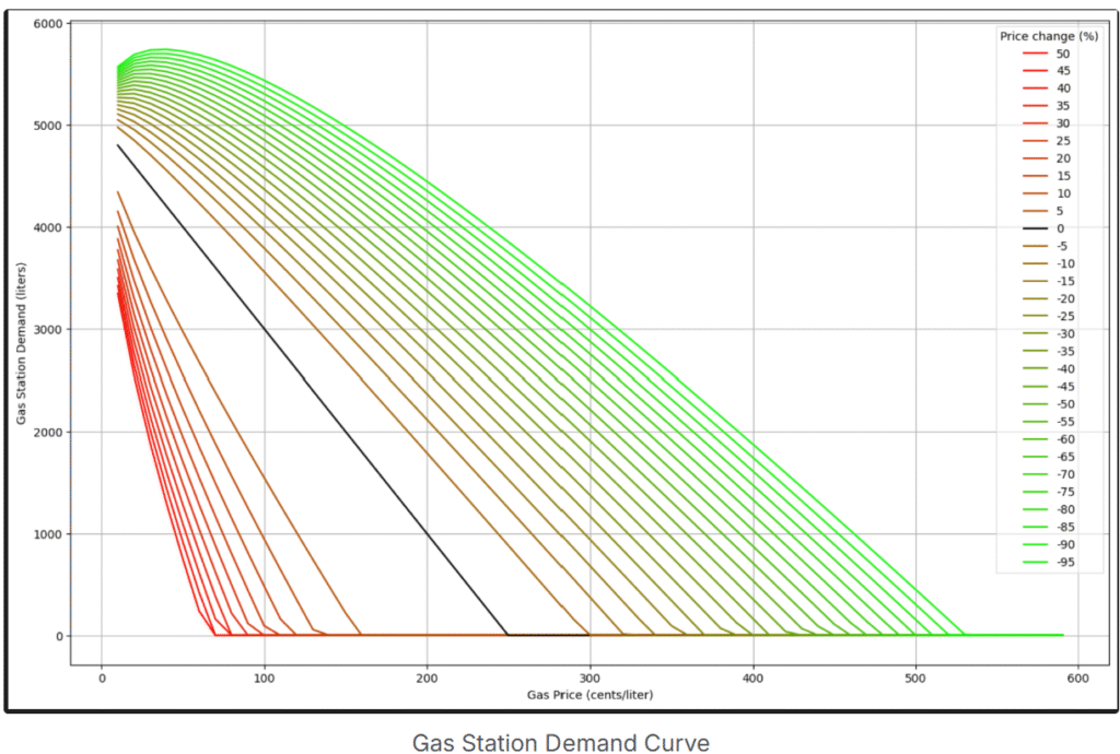
In this environment:
• The gas station can lower its price to increase demand, but prices cannot drop below zero.
• Today’s demand is influenced not only by the current price but also by yesterday’s price, which can lead to counterintuitive outcomes. For example:
• If yesterday’s price was $50/L and today’s price is $20/L, demand may be higher.
• If yesterday’s price was $5/L and today’s price is $10/L, demand may be lower.
Although this environment is simplified compared to real-world markets, it remains non-trivial, providing a meaningful scenario for the Deep RL agent to learn strategies that maximize both demand and profit.

Gas Station Profit Environment
The profit environment is similar to the demand environment, with the key difference that the reward signal is based on profit rather than demand. The Deep Q-Learning agent interacts with this environment to learn strategies that maximize overall profit.

Reinforcement Learning Template
This template follows a single-repo structure for reinforcement learning projects:
• Both training and inference code reside in the same repository, which contains separate pipelines for each.
• Folder-based triggers are configured so that changes under the train or inference folder trigger the corresponding pipeline.
• Dev, PreProd, and Prod accounts are fully isolated, with all necessary AWS resources replicated across accounts.
This structure is particularly suitable for time-series-based forecasting, such as demand and profit optimization in this template. Models are retrained on the latest data, as optimizing tomorrow’s price based on today’s information yields the best results. The fully isolated account structure allows teams to safely make changes in Dev and PreProd while the Production environment continues to serve live traffic.

CI/CD Pipeline
The project includes three pipelines:
• Training Pipeline – Handles model training.
• Inference Pipeline – A self-mutating pipeline for model inference.
• Master Pipeline – Manages project creation and reset (recreates the project).

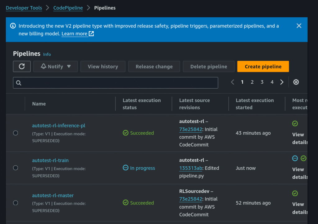
Training – CodePipeline
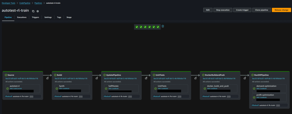
The training CodePipeline, shown below, consists of three key stages:
1. Unit Tests – Validate the training code.
2. Build and Push Docker Images – Three Docker images are built and pushed (details provided in later sections).
3. Model Training Step – Creates two SageMaker pipelines: Demand Optimization and Profit Optimization (described in the next section).

SageMaker Pipelines
This project includes two SageMaker Pipelines:
1. Demand Optimization – Trains a model to maximize gas station demand over a specified period.
2. Profit Optimization – Trains a model to maximize gas station profit over a specified period.

The Profit and Demand training pipelines each consist of three steps. The training and evaluation code is packaged within a Docker image (described in the next section):
1. Hyperparameter Tuning – Searches for optimal training parameters.
2. Model Evaluation – Assesses model performance against evaluation metrics.
3. Model Registration – Registers the trained model in the SageMaker Model Registry.

BYOC (Bring Your Own Container)
The training and evaluation steps in the training pipeline execute code packaged within a custom Docker image. The code structure includes three Dockerfiles, as shown below.
A special note about the inference folder: it contains a Dockerfile but no source code. Inference uses the training code from the train folder, but builds the image using the Dockerfile located in the inference folder. This design is intentional—while the training and inference containers share the same codebase, they require different Dockerfile entry points to meet the requirements of hyperparameter tuning tasks.

Hyperparameter Tuning
When building complex machine learning systems, such as deep neural networks, exhaustively testing all possible hyperparameter combination is impractical. Hyperparameter tuning improves productivity by systematically testing multiple configurations and automatically identifying the most promising set of values within specified ranges. Selecting the right parameter ranges is essential for achieving strong results.
In our Deep Q-Learning template, the hyperparameter tuning step is defined as follows:
• Hyperparameter Ranges – Defines the search space. SageMaker runs one training job for each unique combination of hyperparameters.
• Tuning Job Configuration – Configured to run a maximum of 8 training jobs, with up to 4 running concurrently.
• Objective Metric – Set to total_reward. The training code (packaged in Docker) is responsible for logging this value for each epoch. SageMaker’s Hyperparameter Tuner uses the logged values to determine the best-performing job.
The left pane of the diagram shows the job definition, and the right pane shows the associated code implementing this configuration.

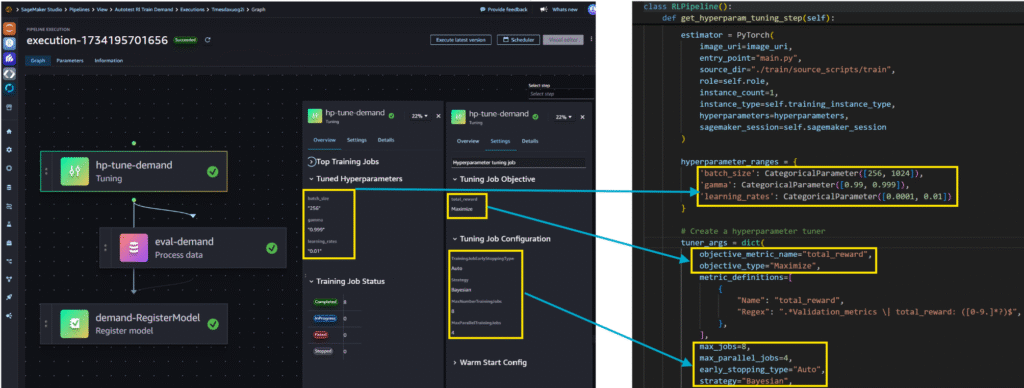
Note: This template uses a restricted hyperparameter search space in the tuning job to reduce compute costs. For more complex Q-Learning problems—where state and action space complexity increases— I recommend expanding the search space to improve results.
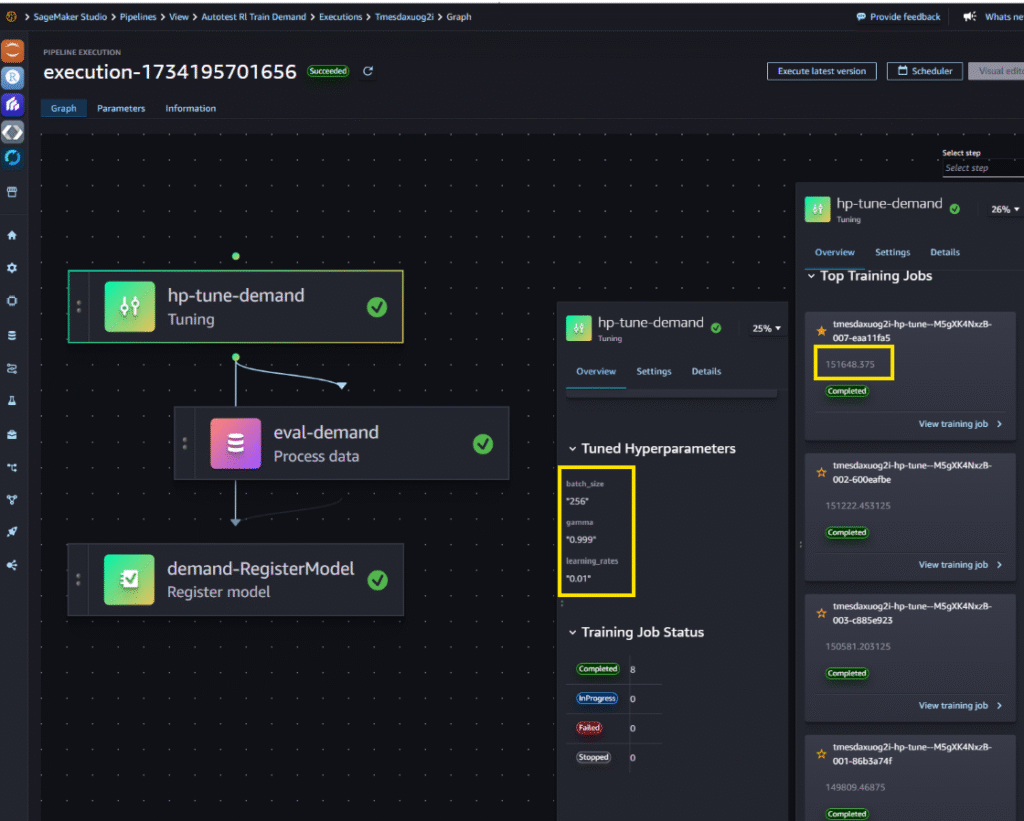
Below is the Hyperparameter Tuning Result. The best-performing configuration is highlighted at the top, followed by the specific hyperparameter values that achieved this result.

Inference
Model Registry
In the Model Registry, Total Reward is used as the primary model quality metric. The examples below illustrate results for the two optimization objectives:
• Left – Demand Optimization: The model achieves an expected volume of 150,971 L, but with a negative profit. This reflects the simple goal of maximizing demand without considering profitability.
• Right – Profit Optimization: The model achieves a profit of $9,798,378 with a significantly lower sales volume.
As this template is based on simplified simulated environment with simplified objectives, these results are intended to demonstrate the reinforcement learning workflow rather than represent real-world operational outcome

Model Approval and Inference Pipeline
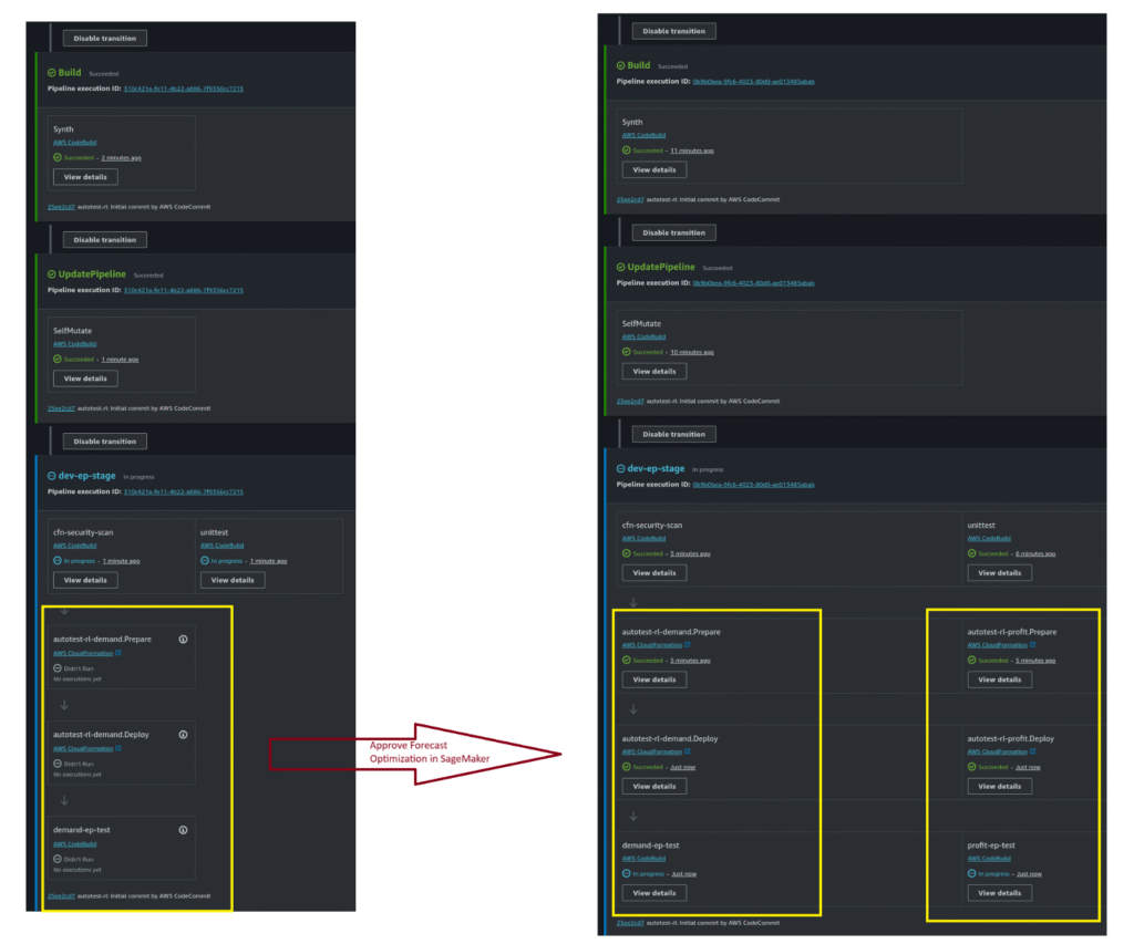
Approving a model version in the Model Registry automatically triggers the Inference Pipeline, as shown below.
The inference pipeline is self-mutating:
• Single Model Approved (left) – If only the demand optimization model is approved, the pipeline contains a single branch.
• Both Models Approved (right) – If both the demand and profit optimization models are approved, the pipeline dynamically expands to include two branches.

Inference Endpoint
When both the demand and profit optimization models are approved, the system deploys two separate SageMaker endpoints: a Demand Endpoint and a Profit Endpoint.
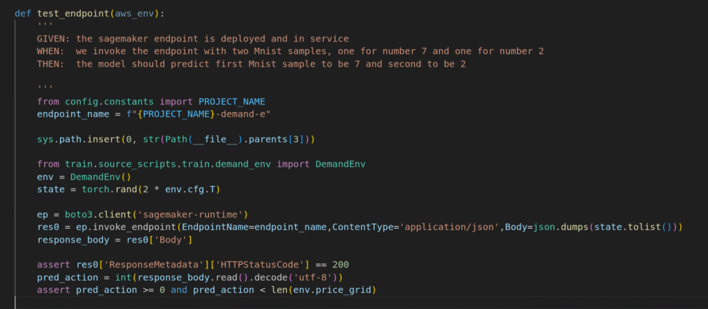
The example below demonstrates testing code for consuming the Demand Endpoint.

Consuming model endpoints
There are two ways to consume the model endpoints:
• When environment of a gas station is not available, use the endpoint to predict tomorrow’s price
• When environment of a gas station is available, I would recommend train the model based on the latest available data (i.e. today’s pricing), then predict the optimal pricing for tomorrow.