Overview
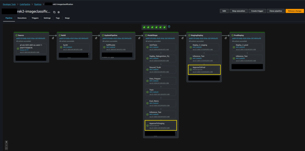
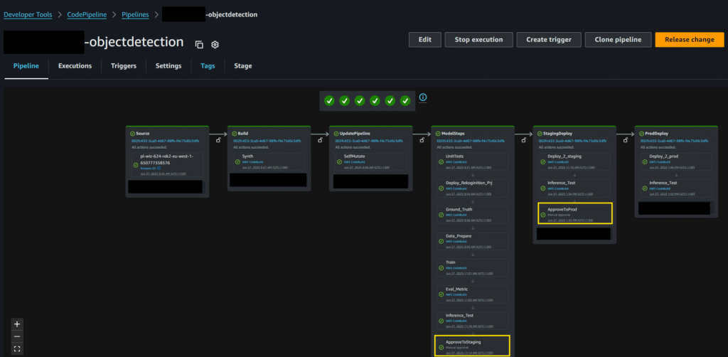
AWS offers 20+ AI services, one of them is Amazon Rekognition. I develop a data science template using Amazon Rekognition to demonstrate how an ML-Ops framework integrates with managed AI services. Packaged as a CloudFormation stack and deployed via AWS Service Catalog, it delivers a fully integrated, end-to-end CI/CD pipeline for image classification and object detection.
The emphasis is on automating the Machine Learning model lifecycle—from data ingestion and model training to model evaluation, model registration, and model deployment—using a repeatable CI/CD pipeline around AWS AI services.
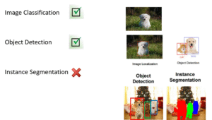
Computer Vision Task
There are three primary types of computer vision tasks:
• Image Classification
• Object Detection
• Instance Segmentation
Amazon Rekognition supports the first two—Image Classification and Object Detection
Ground Truth Strategy
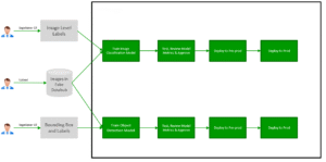
This implementation includes two Amazon Rekognition Custom Labels projects:
• Image Classification
• Object Detection
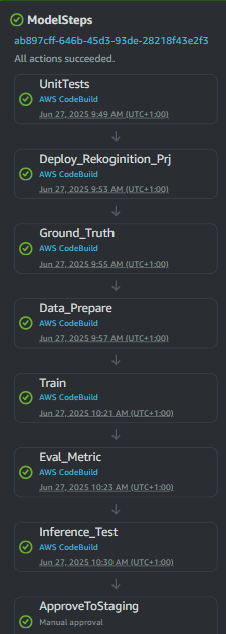
each integrated with its own CI/CD pipeline (as shown below).
Both projects leverage the same image dataset but are annotated with different ground truth labels, defined according to the AWS Ground Truth specification.
CI/CD Pipeline
Both projects are built, trained, and deployed through a CI/CD pipeline, as shown below. The pipeline consists of multiple stages:
1. UnitTests – Runs prior to any deployment. The pipeline halts if tests fail.
2. Deploy – Creates the Rekognition Custom Labels project and provisions required AWS resources (e.g., IAM roles, permissions, S3 buckets).
3. Ground_Truth – Generates ground-truth annotations from the dataset, formatted according to the SageMaker Ground Truth specification, and uploads them to S3.
4. Data_Prepare – Defines the Rekognition training input, including image locations and associated ground-truth data in S3.
5. Training – Initiates training of the Rekognition Custom Labels model.
6. Eval_Metric – Validates model performance against a predefined threshold. If results do not meet the threshold, the pipeline fails.
7. Inference_Test – Performs inference with the trained model. The pipeline fails if inference is unsuccessful or if accuracy falls below the required threshold.
8. Approve2Staging – Upon successful tests and validation, the model is approved for deployment into the Staging environment.
Data Set
We use a dataset of transistor images for training. The dataset is annotated into five classes:
Positive classes (defect types):
• bent_lead – transistor lead is bent
• cut_lead – transistor lead is cut or missing
• damaged_case – visible damage on the transistor case
• misplaced – transistor is misplaced or misaligned
Negative class (normal):
• normal – transistor with no defects
This setup enables the Rekognition Custom Labels models to distinguish between defective and non-defective transistors, supporting both image classification and object detection use cases.
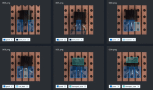
All data are stored in the data-source bucket: s3://…/rekognition/. The folder hierarchy is as following:
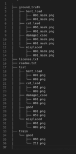
Note that both image classification and object detection use the same images with different ground truth.
Image Classification Ground Truth
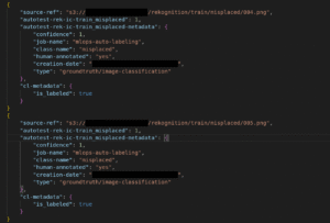
For image classification, the ground truth is defined at the image level. It is automatically generated from the folder structure, following the AWS SageMaker Ground Truth specification. Below is an example shows image classification ground truth of two images:
Object Detection Ground Truth
For object detection, the ground truth is defined at the bounding box level.
Since the original dataset only contained pixel-level masks, we created a conversion function to automatically generate bounding boxes from those masks.
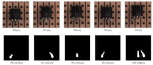
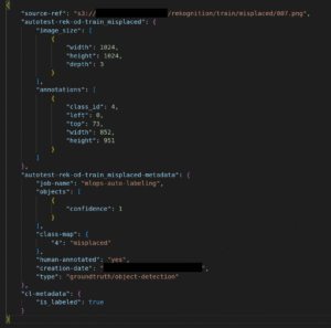
Each bounding box represents the location of a detected defect within the image. The coordinates follow the AWS Ground Truth specification:
• left, top → normalized position of the bounding box (top-left corner).
• width, height → normalized size of the bounding box.
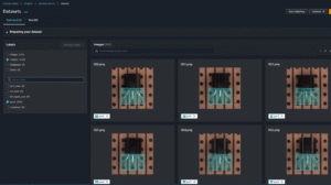
Training Dataset with Ground Truth Overlay
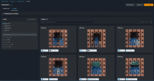
To validate our bounding box generation process, we overlayed the ground truth annotations directly onto the training images. This allows us to visually confirm that each defect is correctly captured and labeled.
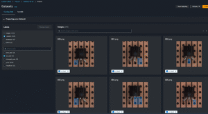
Training Dataset – Positive Samples
To illustrate the quality and diversity of the dataset, below are positive training samples representing each defect class:
Bent Lead – legs of the transistor bent or misaligned.
Cut Lead – missing or shortened legs.
Damaged Case – visible cracks, chips, or surface damage.
Misplaced – incorrectly positioned components.
Testing Dataset
Testing dataset follows the same structure as the training set but contains images that the model has never seen before. This ensures unbiased evaluation of classification and detection accuracy.
The testing dataset includes positive samples (bent_lead, cut_lead, damaged_case, misplaced) and negative samples (normal).
Each test image is annotated with the correct ground truth label (image-level for classification, bounding-box level for detection).
Result Evaluation
Once training is complete, the Rekognition Custom Labels service produces an evaluation report that summarizes model accuracy against the testing dataset. The CI/CD pipeline automatically retrieves these metrics and applies pre-defined thresholds to determine if the model is production-ready.
Key metrics considered:
• Precision – the proportion of correctly identified defects among all predicted defects.
• Recall – the proportion of actual defects correctly identified by the model.
• F1 Score – the harmonic mean of precision and recall, providing a balanced view of performance.
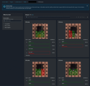
Image Classification Result
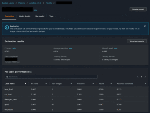
Image Classification Performance
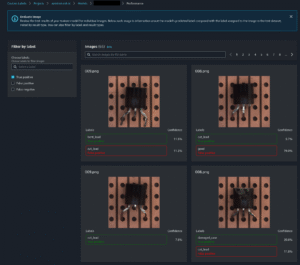
Object Detection Result
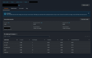
Object Detection Performance
Staging and Production Deployment
Once the training, evaluation, and integration tests have passed, the client can approve the model for deployment to the Staging environment, followed by Production.
After deployment, we perform inference testing with similar approach.
